DIFFRACTIVE MULTIFOCAL INTRODUCTION
A diffractive Multifocal (MF) Lens allows a single incident beam to focus simultaneously at several focal lengths along the propagation axis. The number of foci is determined during the design according to the customer’s application requirements. This application note is meant to aid the user’s understanding of the functionality and considerations when using a diffractive Multifocal element.
OPERATION PRINCIPLE:
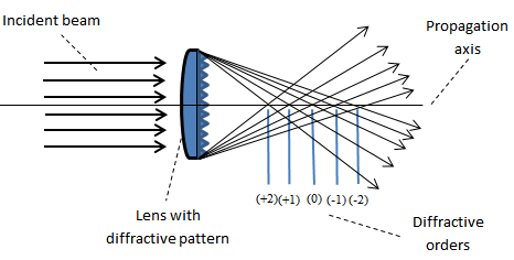
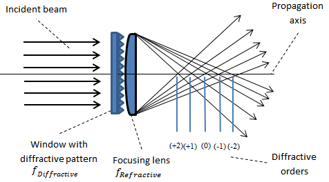
The operational principle is quite straightforward. From a collimated input beam (single mode or multi-mode), the output beam is focused at a fixed number of focal lengths that is predetermined during the design of the DOE based on the customer’s system requirements (See figure 1 and 2 below).
The diffractive Multifocal DOE comes in two configurations:
- DOE that consists of a Plano convex lens with predetermine focal lengths. Here the diffractive pattern is etched on the Plano side. See figure 1 below.
- The other configuration is a diffractive Multifocal that consists of a window which is tailored to the customer’s needs to get a focal point at a certain distance. This is easily achieved by the addition of a simple focusing lens after the DOE, whose BFL (back focal length) determines the working distance (WD). See figure 2 below.
Use Holo/Or’s diffractive Multifocal optical calculator to find the minimum input beam recommended to achieve your desired output, and the different Foci locations.
THEORY:
The multifocal spots’ locations are a function of refractive focal length fRefractive and predetermined diffractive focal length fDiffractive
The foci spot at the “zero” order refers to the refractive focal length of the lens being used.
The other diffractive focal points, orders +/-1,2,3…, appear symmetrically around the refractive “zero” order. An approximation of the distance between the focal points can be described by the equation below:
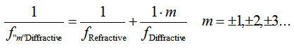
f“m”: Focal Length for “m” diffractive order
fRefractive: Focal Length (FL) of the refractive lens
fDiffractive: FL of the diffractive lens
m: order of multi-focal spot
In the case of an optical set-up using several lenses or thick lenses, please contact Holo/Or for a detailed design. For a multifocal DOE with an even number of foci, the disappearance of the zero order is achieved through special design and processing.
DESIGN CONSIDERATIONS AND LIMITATIONS:
For binary designs (2-level etching), power efficiency can vary between 75% (for Bifocal and multifocal) to 85% (Trifocal) due to physical constraints.
Multi-level etching isn’t always recommended due to manufacturing limitations.
For initial testing purposes, a user may want to use a standard product whose design wavelength (nominal wavelength) is not equal to the wavelength meant for the user’s application. In such a case the defective order FL will change according to the equation:
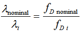
λnominal: The nominal wavelength
λi: Wavelength used by the user
fD nominal: Diffractive Focal Length (FL) for a nominal wavelength
fD i: Diffractive FL for the wavelength used by the user.
In such cases, Holo/Or can simulate the expected performance (power distribution among orders) with the user’s alternative wavelength. Each focal spot contains a fraction of the input beam power.
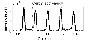
For example, for a trifocal DOE (~85% efficiency), the first focal spot will have around 28% of the input beam power at precise diffractive FL, “+1” order. Moving forward on the propagation axis, a focus will appear at the nominal FL of the lens. Here again the focus spot will have around 28% of the input beam power. The last focus appears at the “-1” order (diffractive order), also with about 28% of the input beam power. At each focal plane, the rest of the power is spread around the focus in the form of a halo.
The minimum input beam size is determined by various design parameters specific to the application at hand, and its diameter must be at least as big as the first 3 Fresnel rings in the DOE.
SIMULATED EFFECTS OF THE INTENSITY DISTRIBUTION ALONG THE PROPAGATION AXIS:
CHANGE OF DISTANCE BETWEEN FOCI
Due to manufacturing limitations or application requirements, sometimes it is required to alter the separation between foci. The simplest way to do this is to change the Effective Focal Length (EFL) of the optical system. Separation between two neighboring foci can be calculated by using the following formula:
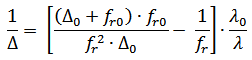
Where:
- Δ: separation between foci
- Δ0: initial separation between foci
- λ: operating wavelength
- λ0: initial wavelength
- fr: EFL of the system after adding additional lens
- fr0 initial EFL of the system
The same mathematical relation can be used for manufacturing semi standard multifocal lenses for specific wavelengths. In this case λ ≠ λ0
Click here for standard diffractive Multifocal products.